Lets face it, robots are cool.
Im joking of course, butonly sort of.
It’s free, every week, in your inbox.
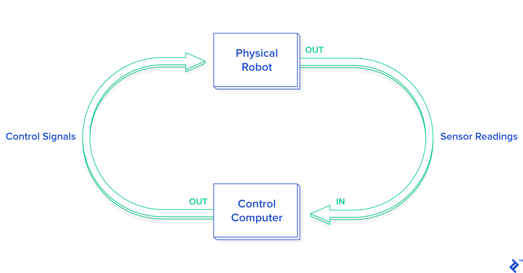
Robot control software can only guess the state of the real world based on measurements returned by its sensors.
It can only attempt to change the state of the real world through the generation of control signals.
Often, once control is lost, it can never be regained.

(Unless some benevolent outside force restores it.)
This is one of the key reasons that robotics programming is so difficult.
Many advances in robotics come from observing living creatures and seeing how they react to unexpected stimuli.
What is your internal model of the world?
It is different from that of an ant, and that of a fish?
However, like the ant and the fish, it is likely to oversimplify some realities of the world.
Sometimes we call this danger.
The same way our little robot struggles to survive against the unknown universe, so do we all.
This is a powerful insight for roboticists.]
In other words, programming a simulated robot is analogous to programming a real robot.
However, I encourage you to dive into the source and mess around.
The simulator has been forked and used to control different mobile robots, including a Roomba2 fromiRobot.
Likewise, like feel free to fork the project and improve it.
For example, think of it driving through multiple waypoints.
However, to complicate matters, the environment of the robot may be strewn with obstacles.
The robot MAY NOT collide with an obstacle on its way to the goal.
The programmable robot
Every robot comes with different capabilities and control concerns.
Lets get familiar with our simulated programmable robot.
Our robot must figure out for itself how to achieve its goals and survive in its environment.
This proves to be a surprisingly difficult challenge for novice robotics programmers.
These can include anything from proximity sensors, light sensors, bumpers, cameras, and so forth.
In addition to the proximity sensors, the robot has a pair of wheel tickers that track wheel movement.
Turns in the opposite direction count backward, decreasing the tick count instead of increasing it.
Later I will show you how to compute it from ticks with an easy Python function.
Control Outputs: mobility
Some robots move around on legs.
Some roll like a ball.
Some even slither like a snake.
Our robot is adifferential driverobot, meaning that it rolls around on two wheels.
When both wheels turn at the same speed, the robot moves in a straight line.
When the wheels move at different speeds, the robot turns.
But if you are curious, I will briefly introduce it here.
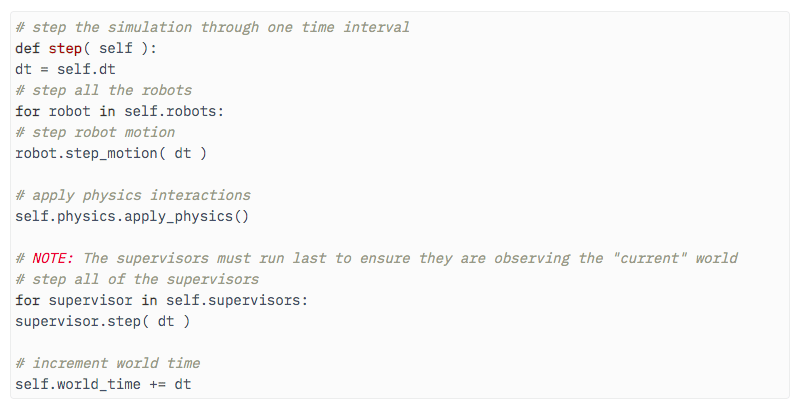
The fileworld.pyis a Python class that represents the simulated world, with robots and obstacles inside.
The same concepts apply to the encoders.
A simple model
First, our robot will have a very simple model.
It will make many assumptions about the world.
A robot is a dynamic system.
The more times we can do this per second, the finer control we will have over the system.
Remember our previous introduction about different robot programming languages for different robotics systems and speed requirements.
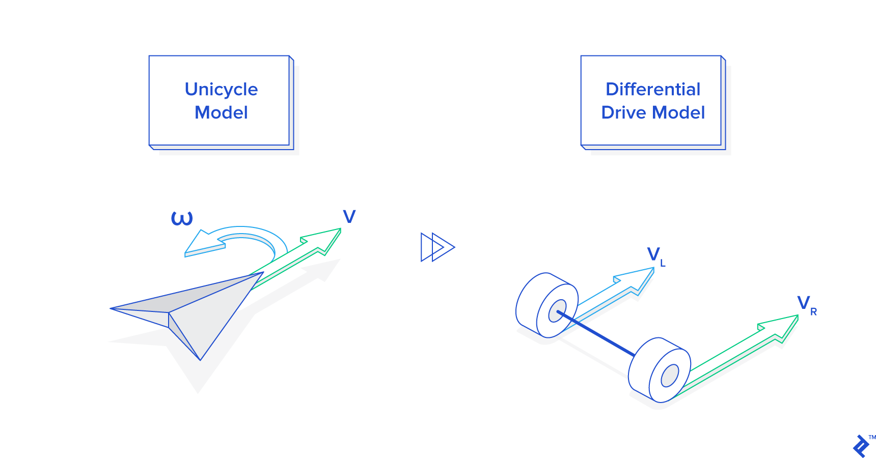
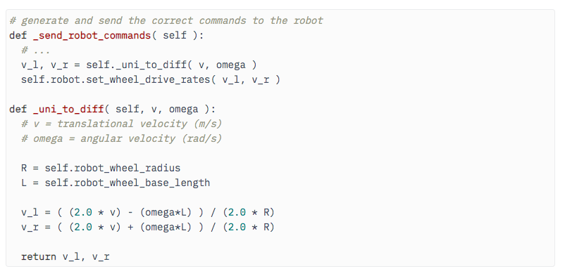
Lets call these signalsvLandvR.
However, constantly thinking in terms ofvLandvRis very cumbersome.
Lets call these parameters velocityvand angular (rotational) velocity(read omega).
This is known as aunicycle modelof control.
Here is the Python code that implements the final transformation insupervisor.py.
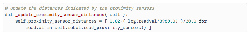
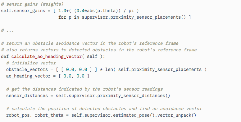
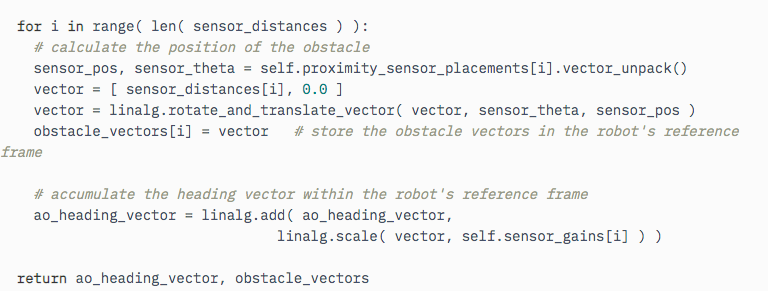
The API functionread_proximity_sensors()returns an array of nine values, one for each sensor.
If there is no obstacle, the sensor will return a reading of its maximum range of 0.2 meters.

Thus, the Python function for determining the distance indicated must convert these readings into meters.
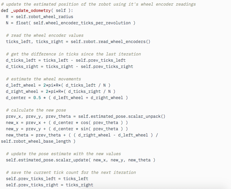
Our robot usesodometryto estimate its pose.
This is where the wheel tickers come in.

Below is the full odometry function insupervisor.pythat updates the robot pose estimation.
Positivexis to the east and positiveyis to the north.
Thus a heading of0indicates that the robot is facing directly east.

The robot always assumes its initial pose is(0, 0), 0.
So how do we make the wheels turn to get it there?
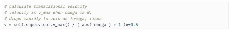
Lets start by simplifying our worldview a little and assume there are no obstacles in the way.
This then becomes a simple task and can be easily programmed in Python.
If we go forward while facing the goal, we will get there.
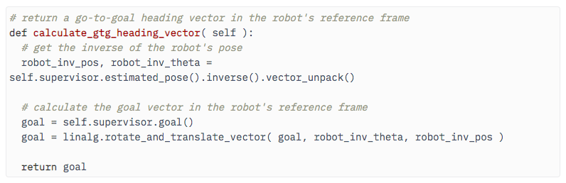
Thanks to our odometry, we know what our current coordinates and heading are.
We also know what the coordinates of the goal are because they were pre-programmed.
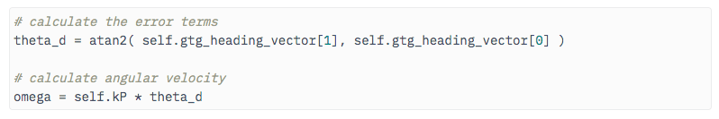
In other words, it is theerrorbetween our current state and what we want our current state to be.
If the error in our heading is0, then the turning rate is also0.
Now that we have our angular velocity, how do we determine our forward velocityv?
This generally helps us keep our system stable and acting within the bounds of our model.
Thus,vis a function of.
How would this formula change?
It has to include somehow a replacement ofv_max()with something proportional to the distance.
OK, we have almost completed a single control loop.
It is an internal representation of where we want to go.
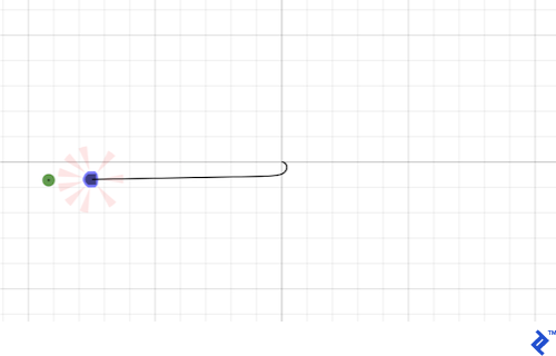
When an obstacle is encountered, turn away from it until it is no longer in front of us.
Thenwill be zero andvwill be maximum speed.
The solution we will develop lies in a class of machines that has the supremely cool-sounding designation ofhybrid automata.
The solution was calledhybridbecause it evolves both in a discrete and continuous fashion.
Our Python robot framework implements the state machine in the filesupervisor_state_machine.py.
When an obstacle is detected, switch to the avoid-obstacles behavior until the obstacle is no longer detected.
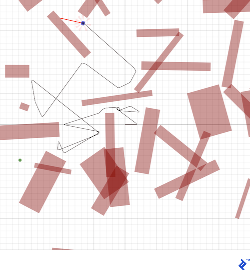
As it turns out, however, this logic will produce a lot of problems.
The result is an endless loop of rapid switching that renders the robot useless.
Then, simply set our reference vector to be parallel to this surface.
Then we can be certain we have navigated the obstacle properly.
To make up our minds, we choose the direction that will move us closer to the goal immediately.
Take a look at the Python code infollow_wall_controller.pyto see how its done.
Final control design
The final control design uses the follow-wall behavior for almost all encounters with obstacles.
Once obstacles have been successfully negotiated, the robot switches to go-to-goal.
Robotics programming often involves a great deal of plain old trial-and-error.
Sometimes it drives itself directly into tight corners and collides.
Sometimes it just oscillates back and forth endlessly on the wrong side of an obstacle.
Occasionally it is legitimately imprisoned with no possible path to the goal.
In the mobile robot universe, our little robots brain is on the simpler end of the spectrum.
Many of the failure cases it encounters could be overcome by adding some more advanced software to the mix.
I hope you will considergetting involvedin the shaping of things to come.
