Machine learning algorithms are used everywhere from a smartphone to a spacecraft.
These algorithms automatically adjust (learn) their internal parameters based on data.
The performance of a model can drastically depend on the choice of its hyperparameters.

The choice of the optimal hyperparameters is more art than science, if we want to run it manually.
Indeed, the optimal selection of the hyperparameter values depends on the problem at hand.
Instead, hyperparameters must be optimized within the context of each machine learning project.
An alternative approach is to set aside the expert and adopt an automatic approach.
A typical optimization procedure treats a machine learning model as a black box.
We do not need (want) to know what kind of magic happens inside the black box.
In this way, the optimization loop runs faster and remains as general as possible.
One further simplification is to use a function with only one hyperparameter to allow for an easy visualization.
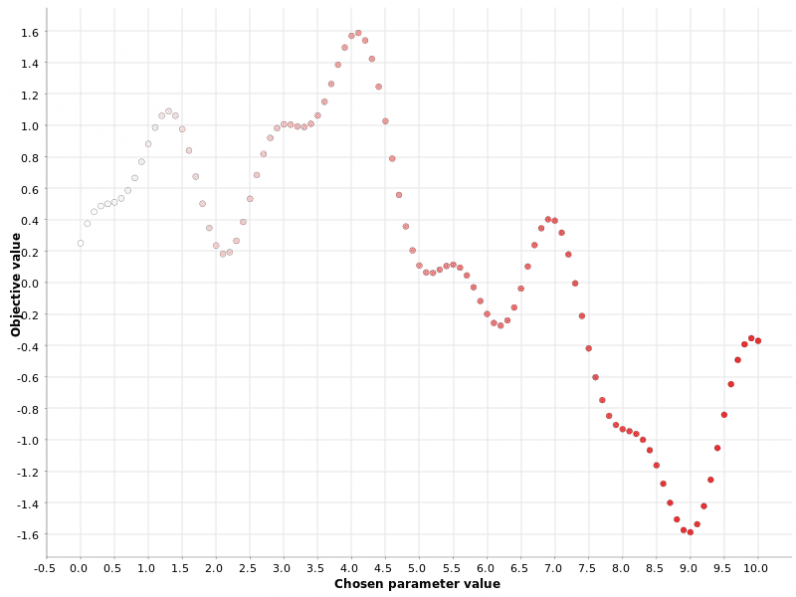
Below is the function we used to demonstrate the four optimization strategies.
We would like to emphasize that any other mathematical function would have worked as well.
On the x axis are the hyperparameter values and on the y axis the function outputs.
This gradient coloring will be useful later to illustrate the differences across the optimization strategies.
Grid search
This is a basicbrute-force strategy.
If you do not know which values to try, you try them all.
All possible values within a range with a fixed step are used in the function evaluation.
The color gradient reflects the position in the generated sequence of hyperparameter candidates.
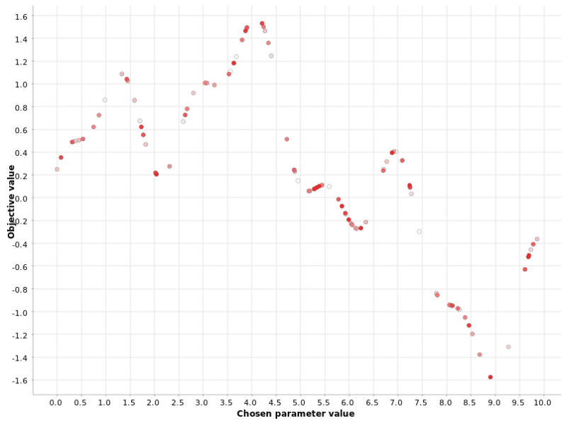
Again, the hyperparameter values are generated within a range [0, 10].
Then, a fixed number N of hyperparameters is randomly generated.
Figure 2: Random search of the hyperparameter values on a [0, 10] range.
The color gradient reflects the position in the generated sequence of hyperparameter candidates.
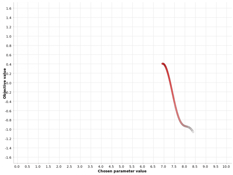
If no neighbor improves the final metric, the optimization loop stops.
Figure 3: Hill climbing search of the hyperparameter values on a [0, 10] range.
The color gradient reflects the position in the generated sequence of hyperparameter candidates.
This example illustrates a caveat related to this strategy: it can get stuck in a secondary maximum.
From the other plots, we can see that the global maximum is located atx=4.0with corresponding metric value of1.6.
This strategy does not find the global maximum but gets stuck into a local one.
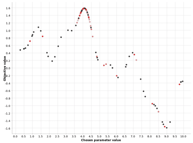
Unlike hill climbing, Bayesian optimization looks at past iterations globally and not only at the last one.
The color gradient reflects the position in the generated sequence of hyperparameter candidates.
This demonstrates that the definition of the optimal region is improved with each iteration of the second phase.
Summary
We all know the importance of hyperparameter optimization while training a machine learning model.
At the end, the hyperparameter set corresponding to the best metric score is chosen as the optimal set.
Now you are all set to go and try them out in a real-world machine learning problem.
